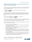
Emerging Practices for Capital Adequacy © Copyright 2003, CCRO. All rights reserved. 70 APPENDIX B: DETAILED EXAMPLE OF THE CALCULATION OF THE CREDIT CAPITAL REQUIREMENT For a Merton model of an infinite portfolio using a single market factor, the expected portfolio losses at X% confidence interval equals the expected loss, conditional on the market variable being at the X% downside confidence interval. In a single factor Merton model (as with any CAPM model), the return for each firm is: ) N( Mkt firm Z )* R (1− Z * R Z 0,1 + = In the above formula, the Z variables represent random variables normally distributed for a specific firm, the market as a whole (i.e. it represents a systematic risk factor), and an error term. R is the pairwise asset correlation so that the square root of R is the correlation of the firm’s assets with the market. Using this modeling foundation, the capital requirement can be estimated as: )] R (1− ))/ Mkt G( * R ) PD N[(G( LGD* K + = LGD is the loss given default, PD is the default probability, and Mkt is the probability of a market downside event. N [.] corresponds to the standard normal cumulative distribution. G (.) denotes the inverse cumulative distribution function for a standard normal random variable. Based on this framework, the computation of the capital requirement percentage (can be thought of as the unexpected probability of default) is: 1. Assume LGD is equal to 100% for simplicity. 2. Assume the market variable has a 99.97% downside event. Assuming a normal distribution, that is 3.43 standard deviations21. 3. Assume a pairwise asset correlation (R) of 0.2. Then the correlation of each firm with the market is the square root of 0.2, which is 0.447. 4. Assume a counterparty has an unconditional default probability of 0.1%. This means its unconditional default distance is -3.09. 5. The counterparty default distance shifts by the market move multiplied by the correlation of the counterparty's assets with the market. In this example, the shift is 3.43 x 0.447, which is 1.53. The new default distance is the original default distance less the shift, which would be -3.09 + 1.53, which is -1.56. 6. This conditional default distance is not a Z-score because the standard deviation is not 1.0. We therefore divide by sqrt (1 – R) to cause the standard deviation to 1.0. In the example, we divide -1.56 by sqrt (1 - 0.2), which gives a standardized default distance of -1.74. This corresponds to a capital requirement percentage of 4.1%22. 21 In Excel, this is computed as default distance = normsinv(default probability). 22 In Excel, this is computed as default probability = normsdist(default distance).