Emerging Practices for Capital Adequacy © Copyright 2003, CCRO. All rights reserved. 16 4.3 Exposure Mapping The various components of financial performance whose value can change with price movements must be identified, captured, modeled, and valued. This requires a detailed analysis of the structure, terms and conditions, and nature of an asset/business in order to be meaningful. The first task is to recognize the market risk factors and then define how they affect the exposures and ultimately the value of the asset/business. Such factors include energy prices, interest rates, foreign exchange rates, and volumes. For complex assets/businesses that include optionality, detailed models may be needed to revalue the asset/business as prices move. For less complex assets/businesses whose value compared against price movements is closer to linear, a simple approximation may be used. When identifying the components of financial performance, considering how volume is treated is important. Volume can be treated as a function of market risk factors or as a separate random variable, or it can be held fixed as a constant. From a practical perspective, a variable energy delivery requirement is usually a function of the market risk factor and is included in the determination of economic capital market risk. Conversely, the probability of an asset’s/business’s performance failure is included in the economic capital for operations risk as discussed in Section VI. 4.4 Definition of Underlying Market Price Variable Movement Processes for Measuring Market Risk The underlying driver for measuring market risk is the estimation of price movements over time5. From a statistical perspective, the objective is to determine a distribution of potential market price outcomes. This is accomplished through either an analytical or simulation-based solution. 4.4.1 Closed-Form Analytical Approach The analytical approach is a closed-form estimation of the distribution of price movements over the desired time horizon. These techniques do not rely on an actual observed distribution they use log normal distribution assumptions to estimate the range of probable market price outcomes for an appropriate confidence level. For example, assuming that daily price returns follow a normal distribution and prices are lognormal, the potential change in gas prices over the next month with a given confidence level can be estimated as follows: • A 95% confidence level is equivalent to 1.65 standard deviations in a normal distribution. • If the annual volatility is approximately 45%, then the monthly volatility is 12.99% (45%*1/12) and the daily volatility is 2.90% (12.99%*1/20) assuming 20 trading days in a month. • Monthly returns are then expected to fluctuate, with a 95% confidence level, between 21.4% (i.e., 1.65*12.99%). 5 Movement in market price variables is typically measured in terms of absolute price changes for basis differentials and in terms of relative price changes for “all in” prices (EM: NYMEX, hub and basis).
Purchased by unknown, nofirst nolast
From: CCRO Library (library.ccro.org)