Emerging Practices for Capital Adequacy © Copyright 2003, CCRO. All rights reserved. 35 The following caveats apply when using the above methodology: 1. This computation only captures default risk. It does not capture the change in economic value due to downgrades. Best practice for credit portfolio models is to include both default risk and downgrade risk. A multiplier could be used to include the impact of downgrades as well as defaults. The key driver of this multiplier would be: – Default probability of the counterparties, and – Maturity of the derivative portfolio A variation of this method converts the cumulative default probability over N years into a one-year probability as an estimated of PD. This will provide a higher estimate of default probability for long-term, highly rated loans than just using the 1-year PD. The impact is less for loans with average credit ratings (BBB). The basic statistical rule for computing the constant default probability each period that would result in the required T-year cumulative default probability indicates: ] ))1/ cumulative PD(Tyear [(1− ) PD(1year T 1− = This rule will not provide reasonable results for exposures expiring in less than a year. 2. Assumes that portfolio is diversified across many industries and products for a corporate portfolio. The assumption of an infinite portfolio substantially understates the credit risk if there are large concentrations. In this case, a multiplier would need to be applied to adjust for the concentration. This multiplier might be estimated through simulations of lumpy portfolios. 3. Distribution is a Merton model based distribution. 5.5.2 Estimation of exposure The second step is to measure the exposure to the counterparty in the event of default. This can be estimated in two ways: 1. Mean positive exposure during the first year which is the average exposure based on a calculation where negative credit exposures have been set to zero. In computing required capital, the mean positive exposure needs to be adjusted upwards to account for the uncertainty of exposure across market scenarios (see Section 5.5.3). 2. Total current exposure (Current MTM, Net A/R and Unbilled), incorporating Potential Future Exposure measurement if analytics are available. The calculation of the mean positive exposure can be simplified by assuming that exposure declines linearly over time, starting with the current exposure. If we estimate the average maturity of the transactions as M years, then the average exposure during the first year is: Average exposure during year 1 = Current exposure x (1 - (0.5 / M))
Purchased by unknown, nofirst nolast
From: CCRO Library (library.ccro.org)