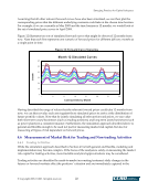
Emerging Practices for Capital Adequacy © Copyright 2003, CCRO. All rights reserved. 22 Assuming that all other relevant forward curves have also been simulated, we can then plot the corresponding prices that the different underlying contracts could take at the chosen time horizon. For example, if we are currently in May 2003 and the time horizon is 12 months, we would look at the set of simulated price curves in April 2004. Figure 12 illustrates ten sets of simulated forward curves that might be observed 12 months from now. Note that each line represents one scenario of forward prices for different delivery months at a single point in time. Figure 12: Forward Curve Scenarios Having described the range of values that the relevant forward prices could take 12 months from now, we can then revalue each asset against these simulated prices to arrive at the distribution of future portfolio values. Note that by jointly simulating all relevant forward prices, we can value both short-term asset/businesses (such as trading positions) and long-term asset/businesses (such as power plants) in a consistent manner. Furthermore, the simulation approach described above is general and flexible enough to be used not just for measuring market risk capital, but also for measuring all types of risk dependent on forward prices. 4.6 Measurement of Market Risk for Trading and Non-trading Activities 4.6.1 Trading Activities While the simulation approach described in Section 4.5 is both general and flexible, modeling and implementation may become complex. If the focus of the analysis is solely on measuring the market risk capital for trading activities, more tractable analytical approximations may be considered. Trading activities are identified by mark-to-market accounting treatment daily changes in the futures or forward markets affect the positions’ valuation and are immediately captured in the Month 12 Simulated Curves 0 10 20 30 40 50 60 1 6 11 16 21 26 31 Contract Delivery Month $/mwh 36