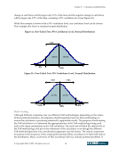
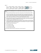
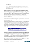
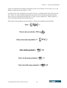
Volume 3 — Valuation and Risk Metrics © Copyright 2002, CCRO. All rights reserved. 49 The Kuiper statistic provides a tool for testing whether the P&L distribution matches that modeled by the VaR method. This is a stronger requirement than just testing whether the 95% requirement is met. A summary of the method: 1. Select a fine grid of probabilities. {0.01, 0.02, ..., 0.99} should be adequate. 2. Each day, calculate the VaR at these levels of confidence. Call them VaR1, VaR2, ..., VaR99. (Note that some of these will be positive and some will be negative.) 3. The following day, record whether the P&L is below each of the calculated values, VaR1, VaR2, ..., VaR99, and keep track of the counts for each probability as N(1), N(2), ..., N(99). 4. After T days (the observation period) calculate Ni/T. 5. Compute the Kuiper statistic: K = max(i) [F(pi) - pi] + max(i) [pi-F(pi)] This has a much higher power than other statistics, is not difficult to calculate, and will quickly indicate whether or not the VaR calculation is working correctly. When using the Kuiper statistic, it is also a good idea to produce a quantile-quantile plot (Q-Q plot). Generally, a Q-Q plot is a tool used to determine if two data sets have a common distribution. The Q-Q plot is a visual illustration of precisely where in the distribution deviations from expectations occur. By generating a Q-Q plot of F(pi) versus a uniform distribution, one can graphically see if the model fits, or identify deviations. Hence, if the Kuiper test fails, the Q-Q plot may help to explain why. (For more detailed discussion on generating and analyzing Q-Q plots, see NIST/SEMATECH e-Handbook of Statistical Methods, www.itl.nist.gov/div898/handbook/eda/section3/qqplot.htm.)