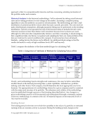
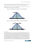
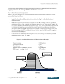
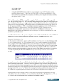
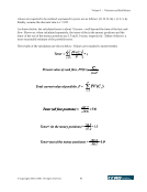
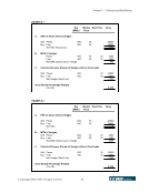
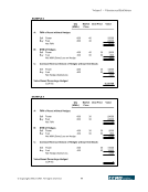
Volume 3 — Valuation and Risk Metrics © Copyright 2002, CCRO. All rights reserved. 47 100*0.9544= 95.44 100*0.0228= 2.28. • Using the CHITEST function with the actual (sample) range of 4, 94, and 2 and the expected (ideal) range of 2.28, 95.44, and 2.28 yields a chi-square probability of .5082. The CHIINV function with the probability of .5082 and two degrees of freedom yields a chi-square value of 1.3537. Note that the number of P&L swings below negative VaR exceeds what would be expected. Also, the chi-square value is not zero, indicating that the distribution does not exactly match the ideal distribution. Therefore, we might reject the null hypothesis that the observed distribution represents the ideal distribution and perhaps replace our method of calculating VaR. However, the chi-square probability of .5082 is much higher than the significance level of 0.05 indicating that this distribution is representative of the ideal distribution. The difference in the distributions is explained by randomness in the observed distribution. In this case, the randomness is the random movements in the forward price curve. We conclude that the VaR calculation is probably sound. For further information on chi-square tests, please refer to statistical textbooks such as Statistical Analysis for Decision Making, by Morris Hamburg, Harcourt, Brace & World, Inc., 1970. Binomial Distribution Test For the purpose of discussion, assume a 95% confidence interval and a one-day holding period. For back-testing purposes, the 95% confidence level is an average companies should observe many samples of the VaR and P&L series to assess the right coverage by counting the number of VaR violations. In this example, we only have one series for the P&L and one corresponding series for VaR. To illustrate the problem, consider drawing samples of 250 values each from a standard normal distribution and counting how many values in each sample are in the lower 5 percentile implied by the theoretical distribution (i.e., how many numbers are lower than - —1.645). Sample I II III IV V VI VII VIII IX X Average Numbers lower than –1.645 9 15 10 12 15 11 15 12 14 8 12.1 Percentage out of 250 3.60 6.00 4.00 4.80 6.00 4.40 6.00 4.80 5.60 3.20 4.84 All samples come from the same distribution, but they do not reproduce exactly the percentiles of the underlying distribution. Therefore, even if we observe a VaR coverage different from 5%, the model and the distribution assumptions may still be correct. Companies should rely on tests of statistical significance of the difference between the observed coverage level and the expected coverage level of 5%. Let  = x/T denote the coverage level calculated from the data, where x is the number of exceptions (number of times P&L is less than VaR) and T is the sample size. The test results for the coverage accuracy of the VaR methodology are presented in the two tables below. Since the test statistics are lower than the critical values, the hypothesis  = 5% is not rejected. The VaR estimates can be considered acceptably accurate.