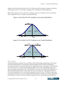
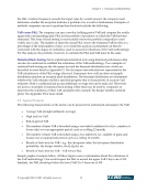
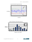
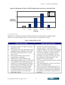
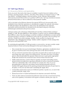
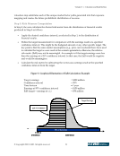
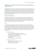
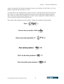
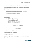
Volume 3 — Valuation and Risk Metrics © Copyright 2002, CCRO. All rights reserved. 46 APPENDIX D – VaR BACK-TESTING METHODOLOGIES Chi-Square Test Description The chi-square test measures how well an observed sample distribution matches an assumed ideal distribution. The VaR calculation for a confidence level of two standard deviations (two tail) assumes that approximately 95% of the P&L swings will occur within plus or minus the VaR value, 2.5% will occur below the negative VaR level, and 2.5% will occur above the positive VaR value. This defines the ideal distribution for the chi-square test. The actual distribution of the P&L swings for the period of study (one year, six months, four months, etc.) is the sample distribution to be tested. A chi-square value of zero indicates a perfect fit to the ideal distribution. The computed value for chi-square is a random variable that takes on different values from sample to sample. As the chi-square values increase, it becomes more questionable whether the sample represents the ideal distribution. The distribution of this chi-square random variable is called the chi- square distribution, which is a function of the number of degrees of freedom. This becomes a hypothesis-testing problem. The null hypothesis is that the ideal distribution describes the sample distribution. A significance level is selected for rejecting the null hypothesis. The significance level is the area under the right-hand tail of the chi-square distribution evaluated at the chi-square value. This involves a tradeoff between a Type I error (incorrectly rejecting the null hypothesis) and a Type II error (incorrectly accepting the null hypothesis). Significance levels are generally set at 0.05 or 0.01 to minimize the potential for Type I errors. Calculation The calculations assume the use of Microsoft® Excel functions CHITEST and CHIINV. CHITEST provides the area under the right-hand tail of the chi-square distribution, and CHIINV provides the chi-square value given the CHITEST result and the number of degrees of freedom. This calculation will be based on a one day, two-tail, two-standard-deviation parametric VaR calculation. The chi-square test as structured will have two degrees of freedom. • First select a null hypothesis. In this case, the null hypothesis is that the VaR calculation is representative of the P&L swings observed. • Select a significance level for rejecting the null hypothesis. We will use 0.05 to minimize the potential for Type I error. • The P&L swings for the period of study should be bucketed. Daily P&L swings below negative VaR, swings between positive and negative VaR, and swings above positive VaR are totaled. This will yield three values that represent the observed distribution. For example, these may be 4, 94, and 2 for a 100-day sample. • The ideal distribution is calculated from the sum of the three numbers in the previous step times the probability (assuming a normal distribution and two standard deviations) for each component of the distribution. In this case, the ideal distribution would be: 100*0.0228= 2.28