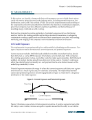
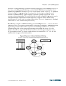
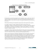
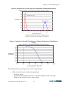
Volume 4— Credit Risk Management © Copyright 2002, CCRO. All rights reserved. 14 The graph highlights the fact that over the given time horizon, exposure can increase or decrease relative to current exposure. Note that for assessing credit risk, one would only be interested in the positive exposures. Calculating Potential Exposure Potential exposure can be calculated at the transaction, counterparty, or portfolio level. The time horizon over which potential exposure is calculated depends on the situation being assessed. For example, potential exposure for a specific deal could be simulated to delivery. At the portfolio level, some companies calculate potential exposure over a one-year period. Ideally, potential exposure should be calculated using a simulation model that re-values the credit portfolio for each outcome. The most sophisticated simulation models would capture price and load uncertainty and accommodate cross-commodity and inter-temporal correlations. Note that simulation models used to calculate VaR can also be used to calculate potential exposure. Interestingly, one can view market risk as being captured by downside VaR while viewing credit risk as being reflected by upside VaR. However, simulating credit exposure would generally be more involved since the calculations need to account for the drop-off in positions that mature during the period being analyzed. To the extent that companies do not have access to simulation models, potential exposure can be approximated using parametric VaR calculated for each counterparty (i.e., counterparty VaR). Counterparty VaR measures how MTM exposure to specific counterparties can change for a given time horizon and confidence level. Counterparty VaR can be converted to potential exposure by accounting for netting and other adjustments described above. This approximation is meaningful when looking at potential exposure to each counterparty independently of the portfolio. Note, however, that adding the potential exposure at each percentile across all counterparties will overstate the portfolio’s true potential exposure, since counterparty exposures are not likely to vary in the same direction at the same time. 2.0 Distribution of Losses Given Default A loss distribution captures the risk that a company could lose money as a result of counterparty default. Calculating a loss distribution requires information on default probabilities, potential exposure, and recovery rates. A default probability indicates the likelihood that a counterparty will fail over a given time horizon. To arrive at a loss distribution, a default probability must first be assigned to each counterparty. This can be done using proprietary models, commercially available models, or published data from rating agencies. Ideally, default probabilities should reflect the possibility of correlated defaults and credit ratings migration. Accounting for migration is especially important when performing the analysis for long time horizons. A loss distribution can be calculated either at the counterparty or portfolio level. To generate a loss distribution, one can jointly simulate potential exposure and default incidence based on the assigned default probabilities. Note that only positive exposures need to be considered insofar